corrr is a package for exploring correlations in R. It makes it possible to easily perform routine tasks when exploring correlation matrices such as ignoring the diagonal, focusing on the correlations of certain variables against others, or rearranging and visualizing the matrix in terms of the strength of the correlations.
Using corrr
Using corrr starts with correlate(), which acts like the base correlation function cor(). It differs by defaulting to pairwise deletion, and returning a correlation data frame (cor_df) of the following structure:
- A
tblwith an additional class,cor_df - An extra “term” column
- Standardized variances (the matrix diagonal) set to missing values (
NA) so they can be ignored.
To work with further, let’s create a correlation data frame using correlate() from the mtcars data that comes with R:
library(corrr)
d <- correlate(mtcars, quiet = TRUE)
d
#> # A tibble: 11 × 12
#>    term     mpg    cyl   disp     hp    drat     wt    qsec     vs      am
#>    <chr>  <dbl>  <dbl>  <dbl>  <dbl>   <dbl>  <dbl>   <dbl>  <dbl>   <dbl>
#>  1 mpg   NA     -0.852 -0.848 -0.776  0.681  -0.868  0.419   0.664  0.600
#>  2 cyl   -0.852 NA      0.902  0.832 -0.700   0.782 -0.591  -0.811 -0.523
#>  3 disp  -0.848  0.902 NA      0.791 -0.710   0.888 -0.434  -0.710 -0.591
#>  4 hp    -0.776  0.832  0.791 NA     -0.449   0.659 -0.708  -0.723 -0.243
#>  5 drat   0.681 -0.700 -0.710 -0.449 NA      -0.712  0.0912  0.440  0.713
#>  6 wt    -0.868  0.782  0.888  0.659 -0.712  NA     -0.175  -0.555 -0.692
#>  7 qsec   0.419 -0.591 -0.434 -0.708  0.0912 -0.175 NA       0.745 -0.230
#>  8 vs     0.664 -0.811 -0.710 -0.723  0.440  -0.555  0.745  NA      0.168
#>  9 am     0.600 -0.523 -0.591 -0.243  0.713  -0.692 -0.230   0.168 NA
#> 10 gear   0.480 -0.493 -0.556 -0.126  0.700  -0.583 -0.213   0.206  0.794
#> 11 carb  -0.551  0.527  0.395  0.750 -0.0908  0.428 -0.656  -0.570  0.0575
#> # … with 2 more variables: gear <dbl>, carb <dbl>
#> # ℹ Use `colnames()` to see all variable names
Why a correlation data frame?
At first, a correlation data frame might seem like an unnecessary complexity compared to the traditional matrix. However, the purpose of corrr is to help use explore these correlations, not to do mathematical or statistical operations. Thus, by having the correlations in a data frame, we can make use of packages that help us work with data frames like dplyr, tidyr, ggplot2, and focus on using data pipelines. Lets look at some examples:
library(dplyr)

# Filter rows to occasions in which cyl has a correlation of .7 or more with
# another variable.
d %>% filter(cyl > .7)
#> # A tibble: 3 × 12
#>   term     mpg   cyl   disp     hp   drat     wt   qsec     vs     am
#>   <chr>  <dbl> <dbl>  <dbl>  <dbl>  <dbl>  <dbl>  <dbl>  <dbl>  <dbl>
#> 1 disp  -0.848 0.902 NA      0.791 -0.710  0.888 -0.434 -0.710 -0.591
#> 2 hp    -0.776 0.832  0.791 NA     -0.449  0.659 -0.708 -0.723 -0.243
#> 3 wt    -0.868 0.782  0.888  0.659 -0.712 NA     -0.175 -0.555 -0.692
#> # … with 2 more variables: gear <dbl>, carb <dbl>
#> # ℹ Use `colnames()` to see all variable names

# Select the mpg, cyl and disp columns (and term)
d %>% select(term, mpg, cyl, disp)
#> # A tibble: 11 × 4
#>    term     mpg    cyl   disp
#>    <chr>  <dbl>  <dbl>  <dbl>
#>  1 mpg   NA     -0.852 -0.848
#>  2 cyl   -0.852 NA      0.902
#>  3 disp  -0.848  0.902 NA
#>  4 hp    -0.776  0.832  0.791
#>  5 drat   0.681 -0.700 -0.710
#>  6 wt    -0.868  0.782  0.888
#>  7 qsec   0.419 -0.591 -0.434
#>  8 vs     0.664 -0.811 -0.710
#>  9 am     0.600 -0.523 -0.591
#> 10 gear   0.480 -0.493 -0.556
#> 11 carb  -0.551  0.527  0.395

# Combine above in a single pipeline
d %>%
  filter(cyl > .7) %>%
  select(term, mpg, cyl, disp)
#> # A tibble: 3 × 4
#>   term     mpg   cyl   disp
#>   <chr>  <dbl> <dbl>  <dbl>
#> 1 disp  -0.848 0.902 NA
#> 2 hp    -0.776 0.832  0.791
#> 3 wt    -0.868 0.782  0.888
Furthermore, by having the diagonal set to missing, we don’t need to put in extra effort to ignore them when summarizing the correlations. For example:
# Compute mean of each column
library(purrr)
d %>%
  select(-term) %>%
  map_dbl(~ mean(., na.rm = TRUE))
#>           mpg           cyl          disp            hp          drat
#> -0.1050454113 -0.0925483176 -0.0872737071  0.0006800268 -0.0037165212
#>            wt          qsec            vs            am          gear
#> -0.0828684293 -0.1752247305 -0.1145625942  0.0053087327  0.0484120552
#>          carb
#>  0.0563419513
API
As the above section suggests, the corrr API is designed with data pipelines in mind (e.g., to use %>% from the magrittr package). After correlate(), the primary corrr functions take a cor_df as their first argument, and return a cor_df or tbl (or output like a plot). These functions serve one of three purposes:
Internal changes (cor_df out):
-
shave()the upper or lower triangle (set to NA). -
rearrange()the columns and rows based on correlation strengths.
Reshape structure (tbl or cor_df out):
Output/visualizations (console/plot out):
-
fashion()the correlations for pretty printing. -
rplot()a shape for each correlation. -
network_plot()a point for each variable, joined by paths for correlations.
By combing these functions in data pipelines, it’s possible to easily explore your correlations.
For example, lets focus on the correlations of mpg and cyl with all the others:
d %>% focus(mpg, cyl)
#> # A tibble: 9 × 3
#> term mpg cyl
#> <chr> <dbl> <dbl>
#> 1 disp -0.848 0.902
#> 2 hp -0.776 0.832
#> 3 drat 0.681 -0.700
#> 4 wt -0.868 0.782
#> 5 qsec 0.419 -0.591
#> 6 vs 0.664 -0.811
#> 7 am 0.600 -0.523
#> 8 gear 0.480 -0.493
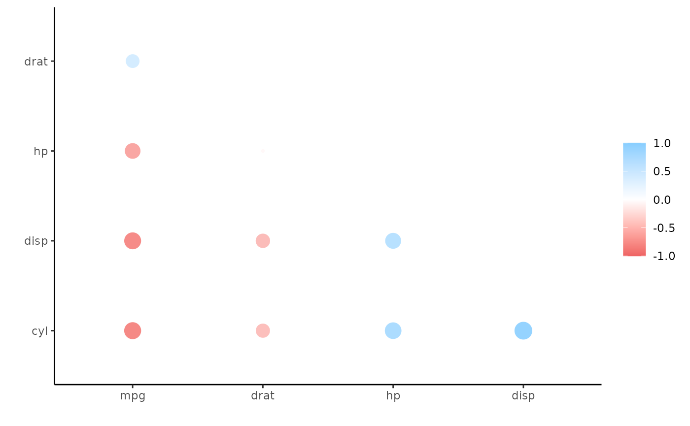
#> 9 carb -0.551 0.527Or maybe we want to focus in on a few variables (mirrored in rows too) and print the correlations without an upper triangle and fashioned to look nice:
d %>%
  focus(mpg:drat, mirror = TRUE) %>%  # Focus only on mpg:drat
  shave() %>% # Remove the upper triangle
  fashion()   # Print in nice format
#>   term  mpg  cyl disp   hp drat
#> 1  mpg
#> 2  cyl -.85
#> 3 disp -.85  .90
#> 4   hp -.78  .83  .79
#> 5 drat  .68 -.70 -.71 -.45
Alternatively, we can visualize these correlations (let’s clear the lower triangle for a change):
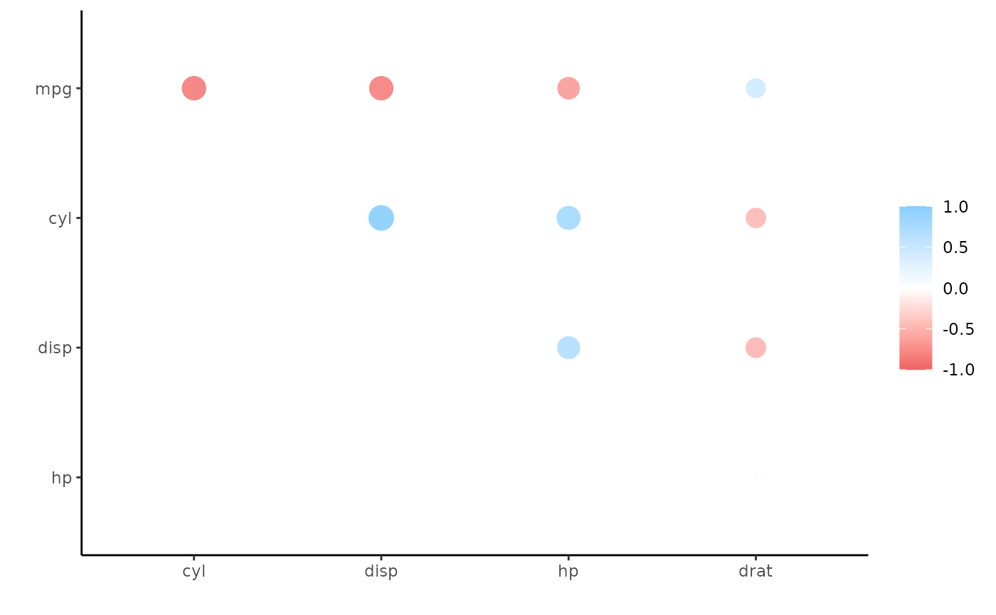
Perhaps we’d like to rearrange the correlations so that the plot becomes easier to interpret. In this case, we can add rearrange() into our pipeline before shaving one of the triangles (we’ll take correlation sign into account with absolute = FALSE).